Basic Examples (2)
Basic Examples
(2)
Generate a Bayesian linear regression on random data:
In[1]:=
Out[1]=
LogEvidence-5.80737,PriorParametersB{0,0},Lambda,0,0,,LambdaInverse{{100,0},{0,100}},V,Nu,PosteriorParametersB{0.621262,0.0167739},Lambda{{2.01,1.12038},{1.12038,0.694701}},LambdaInverse{{4.92336,-7.94014},{-7.94014,14.2449}},V0.014074,Nu,PosteriorRegressionCoefficientDistributionMultivariateTDistribution{0.621262,0.0167739},{{0.0344734,-0.0555969},{-0.0555969,0.0997429}},,ErrorDistributionInverseGammaDistribution,0.00703701,PredictiveDistributionStudentTDistribution0.621262+0.0167739x.,0.0836779,UnderlyingValueDistributionStudentTDistribution0.621262+0.0167739x.,0.0836779,PriorRegressionCoefficientDistributionMultivariateTDistribution{0,0},{{100,0},{0,100}},,ErrorDistributionInverseGammaDistribution,,PredictiveDistributionStudentTDistribution0,,UnderlyingValueDistributionStudentTDistribution0,10,Basis{1,x.},IndependentVariables{x.}
1
100
1
100
1
100
1
100
201
100
201
100
201
200
5.92336-15.8803x.+14.2449
,2
x.
201
100
4.92336-15.8803x.+14.2449
,2
x.
201
100
1
100
1
200
1
200
101+100
,2
x.
1
100
1+
,2
x.
1
100
———
Generate test data:
In[1]:=
data=RandomVariateMultinormalDistribution
,20;ListPlot[data]
1 | 0.7 |
0.7 | 1 |
Out[1]=
Fit the data with a first-order polynomial:
In[2]:=
linearModel=[data,x.,x.]//Keys
Out[2]=
{LogEvidence,PriorParameters,PosteriorParameters,Posterior,Prior,Basis,IndependentVariables}
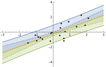
Show the predictive distribution of the model and the distribution of the fit line (dashed):
In[3]:=
Show[Plot[Evaluate@InverseCDF[linearModel["Posterior","PredictiveDistribution"],{0.95,0.5,0.05}],{x.,-3,3},Filling{1{2},3{2}},PlotLegendsTable[Quantity[i,"Percent"],{i,{95,50,5}}]],Plot[Evaluate@InverseCDF[linearModel["Posterior","UnderlyingValueDistribution"],{0.95,0.5,0.05}],{x.,-3,3},Filling{1{2},3{2}},PlotStyleDashed],ListPlot[data,PlotStyleBlack],PlotRangeAll]
Out[3]=
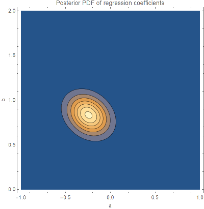
Plot the joint distribution of the coefficients and in the regression equation :
a
b
yax+b
In[4]:=
With[{coefficientDist=linearModel["Posterior","RegressionCoefficientDistribution"]},ContourPlot[Evaluate[PDF[coefficientDist,{a,b}]],{a,-1,1},{b,0,2},PlotRange{0,All},PlotPoints20,FrameLabel{"a","b"},ImageSize400,PlotLabel"Posterior PDF of regression coefficients"]]
Out[4]=
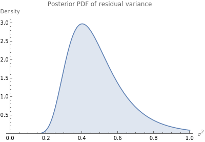
Plot the of the posterior variance of the residuals:
In[5]:=
With[{errDist=linearModel["Posterior","ErrorDistribution"]},Quiet@Plot[Evaluate[PDF[errDist,e]],{e,0,1},PlotRange{0,All},AxesLabel{"","Density"},ImageSize400,FillingAxis,PlotLabel"Posterior PDF of residual variance"]]
2
σ
Out[5]=
Fit the data with a polynomial of arbitrary degree and compare the prediction bands and log-evidence of fits up to degree 4:
In[6]:=
TableModulemodel=[Rule@@@data,x.^Range[0,degree],x.],predictiveDist,predictiveDist=model["Posterior","PredictiveDistribution"];Show[Plot[Evaluate@InverseCDF[predictiveDist,{0.95,0.5,0.05}],{x.,-3,3},Filling{1{2},3{2}},PlotLegendsTable[Quantity[i,"Percent"],{i,{95,50,5}}]],ListPlot[data,PlotStyleBlack],PlotRangeAll,PlotLabelStringForm["Degree: `1`\nLog evidence: `2`",degree,model["LogEvidence"]]],{degree,0,4}