Basic Examples (10)
Basic Examples
(10)
Take random times and corresponding values for the function :
f(t)=sin(t)+cos(3t)/2
In[1]:=
SeedRandom[11222333344444]data=Sort[Map[{#,Sin[#]+Cos[3*#]/2}&,RandomReal[{0,20},500]]];
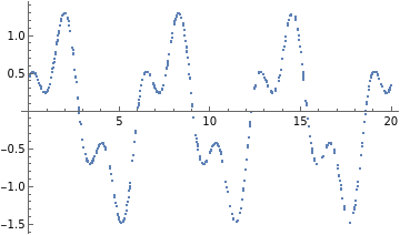
Subtract the mean of the data values and plot the resulting time series:
In[2]:=
times=data[[All,1]];vals=data[[All,2]]-Mean[data[[All,2]]];ListPlot[Transpose[{times,vals}]]
Out[2]=
Plot the periodogram computed from this unevenly spaced set of measurements:
In[3]:=
Plot[w,times,vals],{w,.1,5},PlotPoints300,PlotRangeAll,AxesLabel{"ω (radians)","(ω)"},ImageSize400
P
D
Out[3]=
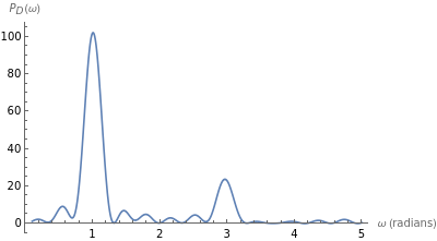
Compute the larger frequency (the location of the larger spike):
In[4]:=
freq=NArgMax[w,times,vals],.7≤w≤1.3,w
Out[4]=
1.00487
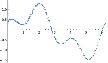
Compute the period from this frequency:
In[5]:=
per=2Pi/freq
Out[5]=
6.2527
Plot the time series "folded" by this period (times are computed modulo the computed period) to see the approximately sinusoidal variation in the light curve:
In[6]:=
foldTimes[times_,period_]:=period*FractionalPart[times/period]
In[7]:=
ListPlot[Transpose[{foldTimes[times,per],vals}]]
Out[7]=
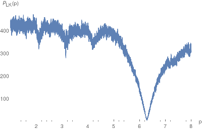
The string-length approach also shows this periodicity:
In[8]:=
Plot[p,times,vals,Method"LaflerKinman"],{p,1,8},PlotPoints300,PlotRangeAll,AxesLabel{"p","(p)"},ImageSize400
P
LK
Out[8]=
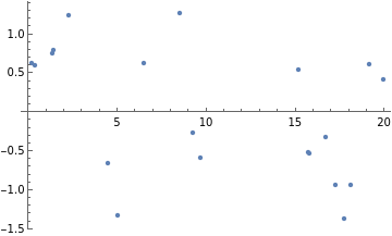
One can get a fairly good estimate of the frequencies present using far fewer samples, so long as they are irregularly spaced in time. Take 20 random points from the preceding original set:
In[9]:=
SeedRandom[11222333344444]data2=Sort[RandomSample[data,20]];times2=data2[[All,1]];vals2=data2[[All,2]]-Mean[data2[[All,2]]];ListPlot[Transpose[{times2,vals2}]]
Out[9]=
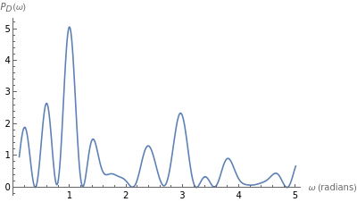
Plot the periodogram from this subset:
In[10]:=
Plot[w,times2,vals2],{w,.1,5},PlotPoints300,PlotRangeAll,AxesLabel{"ω (radians)","(ω)"},ImageSize400
P
D
Out[10]=
Estimate the period for the larger frequency:
In[11]:=
freq=NArgMax[w,times2,vals2],.7≤w≤1.3,w
Out[11]=
0.989728
Scope (2)
Scope
(2)
Properties & Relations (2)
Properties & Relations
(2)
Applications (43)
Applications
(43)